Quadrature
Scott Prahl
January 2021
version 2
[1]:
import numpy as np
import matplotlib.pyplot as plt
import iadpython.quadrature
Adding-Doubling and Quadrature
The adding-doubling method is based on numerical integration of functions using quadrature,
The values of the quadrature points \(x_i\) and the weights \(w_i\) are chosen in such a way that the integral is evaluated exactly for a polynomial of order \(2N-1\) (or possibly \(2N-2\) depending on the quadrature method). Using \(N\) quadrature points (Gaussian) is equivalent to the spherical harmonic method of order \(P_{N-1}\), i.e. four quadrature points corresponds to the \(P_3\) method. The specific choice of quadrature methods for samples with mismatched boundaries is described in the next section.
Total internal reflection causes problems by changing the effective range of integration. Usually, adding-doubling integrals range from \(0\) to \(1\), since the angle varies from \({\pi\over2}\) to \(0\) and therefore the cosine varies from \(0\) to \(1\). The integrations are calculated using numerical quadrature, and the quadrature angles are optimized for this range. If the cosine of the critical angle is denoted by \(\nu_c\) for a boundary layer with total internal reflection, then the effective range of integration is reduced to \(\nu_c\) to \(1\) (because the rest of the integration range is now zero). To maintain integration accuracy, the integral is broken into two parts and each is evaluated by quadrature over the specified subrange,
Here \(A(\nu,\nu')\) and \(B(\nu,\nu')\) represent reflection or transmission functions, and clearly if either is identically zero for values of \(\nu\) less than \(\nu_c\), the integration range is reduced.
Each integral is handled with a different quadrature scheme. Specifically the calculations used Gaussian quadrature for integrals over the range from \(0\) to \(\nu_c\), thereby avoiding calculations at both endpoints (in particular, the angle \(\nu=0\) is avoided, which may cause division by zero).
Radau quadrature is used for the range from \(\nu_c\) to \(1\), so \(\nu=1\) could be specified as a quadrature point. Each part of the integration range gets half of the quadrature points; when no critical angle exists, Radau quadrature is used over the entire range.
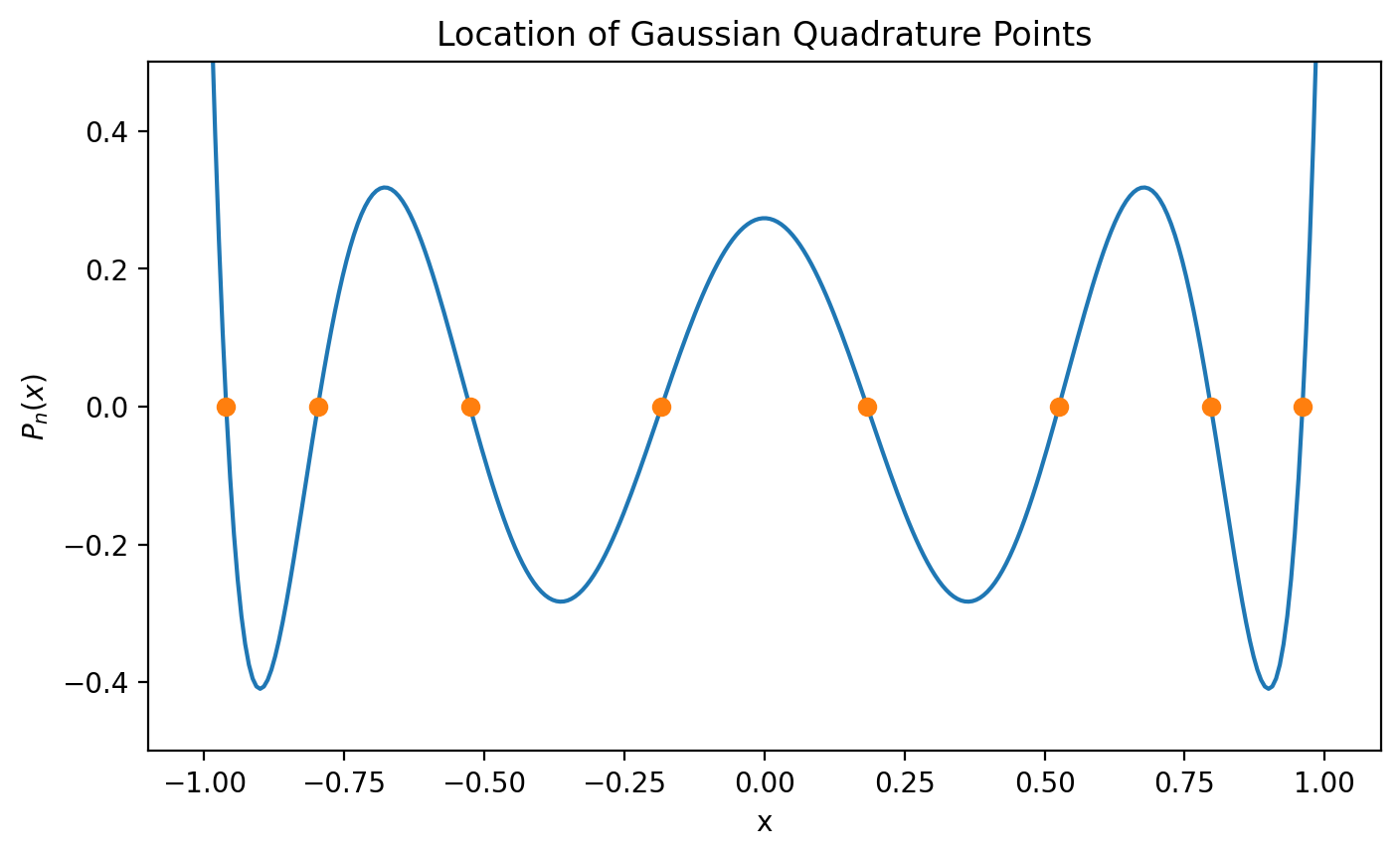
Standard Gaussian-Legendre Quadrature
Gauss nodes \(x_i\) are the roots of the nth Legendre polynomial \(P_n(x)\). The weights \(w_i\) are
[2]:
n=8
xi, wi = iadpython.quadrature.gauss(n)
[3]:
xx=np.empty(8)
ww=np.empty(8)
xx[4]=-0.1834346424956498
xx[3]=0.1834346424956498
xx[5]=-0.5255324099163290
xx[2]=0.5255324099163290
xx[6]=-0.7966664774136267
xx[1]=0.7966664774136267
xx[7]=-0.9602898564975363
xx[0]=0.9602898564975363

ww[4]=0.3626837833783620
ww[3]=0.3626837833783620
ww[5]=0.3137066458778873
ww[2]=0.3137066458778873
ww[6]=0.2223810344533745
ww[1]=0.2223810344533745
ww[7]=0.1012285362903763
ww[0]=0.1012285362903763

ww = np.flip(ww)
xx = np.flip(xx)
print(" i        xi calc         xi ref            wi calc         wi ref")
print("----------------------------------------------------------------------")
for i,x in enumerate(xi):
    print("%2d   %+.12f %+.12f   %+.12f %+.12f" % (i, x, xx[i], wi[i], ww[i]))
 i        xi calc         xi ref            wi calc         wi ref
----------------------------------------------------------------------
 0   -0.960289856498 -0.960289856498   +0.101228536290 +0.101228536290
 1   -0.796666477414 -0.796666477414   +0.222381034453 +0.222381034453
 2   -0.525532409916 -0.525532409916   +0.313706645878 +0.313706645878
 3   -0.183434642496 -0.183434642496   +0.362683783378 +0.362683783378
 4   +0.183434642496 +0.183434642496   +0.362683783378 +0.362683783378
 5   +0.525532409916 +0.525532409916   +0.313706645878 +0.313706645878
 6   +0.796666477414 +0.796666477414   +0.222381034453 +0.222381034453
 7   +0.960289856498 +0.960289856498   +0.101228536290 +0.101228536290
[4]:
x = np.linspace(-1+1e-10, 1-1e-10, 300)
plt.plot(x, iadpython.quadrature._gauss_func(n, x))
plt.plot(xi, iadpython.quadrature._gauss_func(n, xi), "o")
plt.ylim(-0.5,0.5)
plt.xlabel("x")
plt.ylabel('$P_n(x)$')
plt.title('Location of Gaussian Quadrature Points')
plt.show()
[5]:
n=8
xi, wi = iadpython.quadrature.gauss(n,-7,2)

# integral of x^6 from 0 to 2 should be (x^7)/7

quad_int = np.sum(xi**6 * wi)
anal_int = (2)**7 / 7 - (-7)**7 / 7

print(quad_int)
print(anal_int)
117667.2857142855
117667.28571428571
Gauss-Radau Quadrature
Solution for integration range from -1 to 1
Radau quadrature is a Gaussian Quadrature-like formula for numerical estimation of integrals. It requires \(m+1\) points and fits all Polynomials to degree \(2m\), so it effectively fits exactly all Polynomials of degree \(2m-1\). It uses a weighting Function \(w(x)=1\) in which the endpoint \(-1\) in the interval \([-1,1]\) is included in a total of \(n\) Abscissas, giving \(r=n-1\) free abscissas. The general formula is
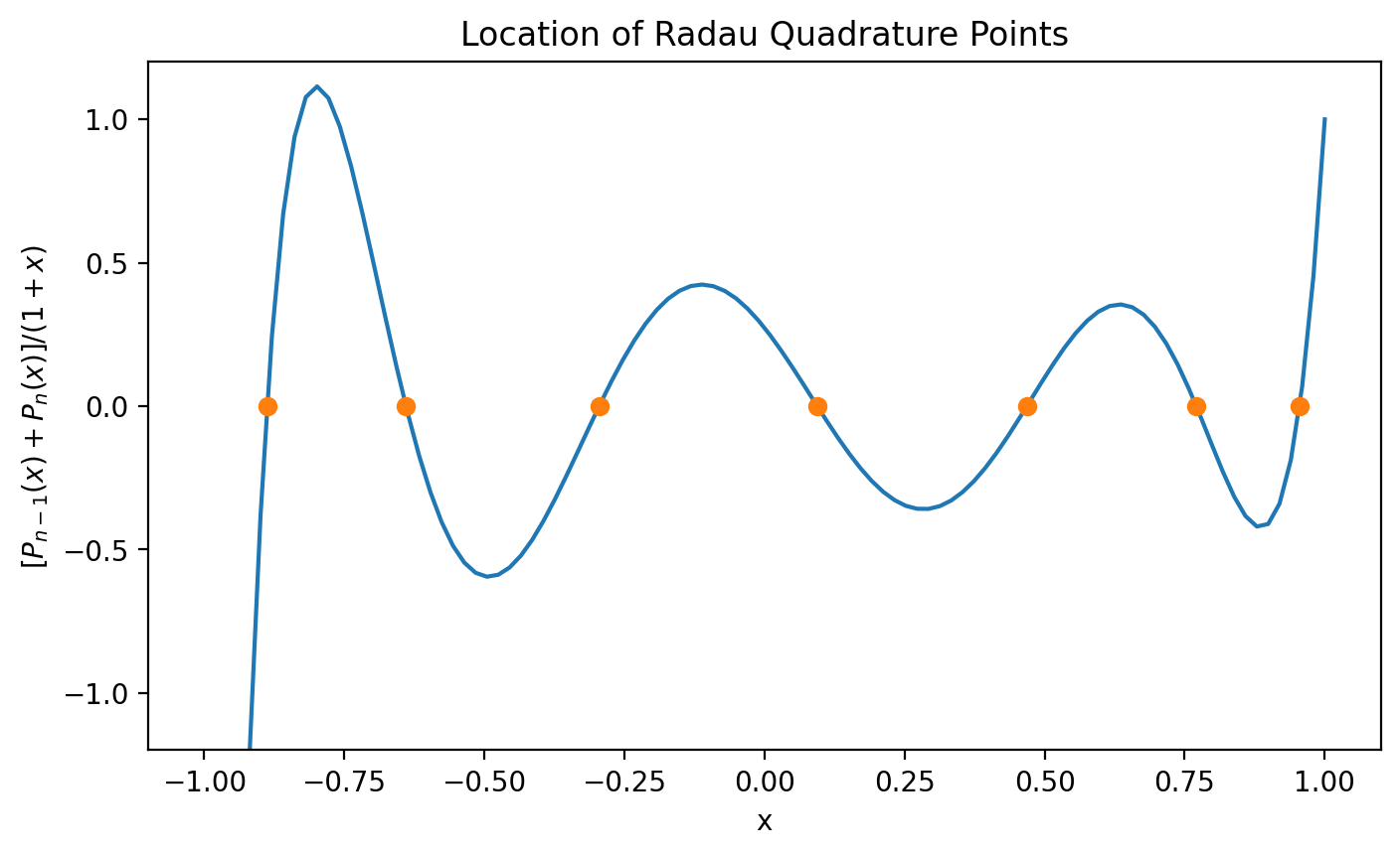
The nodes \(x_i\) are given by the \(n\) roots of
Here \(P_n(x)\) is the \(n\)th Legendre polynomial of order zero and \(P_{n-1}'(x_i)\) is the first derivative of the \((n-1)\)st Legendre polynomial. These roots are the required quadrature points distributed within the integration range \(-1\) to \(1\).
The weights \(w_i=w(x_i)\) are
with
Solution for integration range from a to b
Radau quadrature is defined over the range -1 to 1. The constrained endpoint is usually assumed to be the lower limit of integration or \(-1\). However, we will want the common endpoint to be the upper limit of integration. Furthermore, we want to integrate over an arbitrary range of values so we note
and we do quadrature on the integral on the right hand side
To modify for the range \(a\) to \(b\) the following relations are needed to find the necessary quadrature points \(x_i\) and weights \(w_i\) so that
where the new abscissas and weights are
and
[6]:
n=8
xi, wi = iadpython.quadrature.radau(n)
[7]:
xx=np.empty(8)
ww=np.empty(8)
xx[7]= -1
xx[6]=-0.8874748789261557
xx[5]=-0.6395186165262152
xx[4]=-0.2947505657736607
xx[3]= 0.0943072526611108
xx[2]= 0.4684203544308211
xx[1]= 0.7706418936781916
xx[0]= 0.9550412271225750

ww[7]= 2/(8*8)
ww[6]= 0.1853581548029793
ww[5]= 0.3041306206467856
ww[4]= 0.3765175453891186
ww[3]= 0.3915721674524935
ww[2]= 0.3470147956345014
ww[1]= 0.2496479013298649
ww[0]= 0.1145088147442572

# the provided solutions must be adapted because the lower endpoint is assumed fixed
xx = -xx
print(" i        xi calc         xi ref            wi calc         wi ref")
print("----------------------------------------------------------------------")
for i,x in enumerate(xi):
    print("%2d   %+.12f %+.12f   %+.12f %+.12f" % (i, x, xx[i], wi[i], ww[i]))
 i        xi calc         xi ref            wi calc         wi ref
----------------------------------------------------------------------
 0   -0.955041227123 -0.955041227123   +0.114508814744 +0.114508814744
 1   -0.770641893678 -0.770641893678   +0.249647901330 +0.249647901330
 2   -0.468420354431 -0.468420354431   +0.347014795635 +0.347014795635
 3   -0.094307252661 -0.094307252661   +0.391572167452 +0.391572167452
 4   +0.294750565774 +0.294750565774   +0.376517545389 +0.376517545389
 5   +0.639518616526 +0.639518616526   +0.304130620648 +0.304130620647
 6   +0.887474878926 +0.887474878926   +0.185358154809 +0.185358154803
 7   +1.000000000000 +1.000000000000   +0.031250000000 +0.031250000000
[8]:
eps = 1e-8
x = np.linspace(-1+eps, 1-eps, 100)
plt.plot(x, iadpython.quadrature._radau_func(n, x))
# have to plot -xi because we fix upper endpoint
plt.plot(-xi[:-1], iadpython.quadrature._radau_func(n, -xi[:-1]), "o")
plt.ylim(-1.2,1.2)
plt.xlabel("x")
plt.ylabel('$[P_{n-1}(x)+P_n(x)]/(1+x)$')
plt.title('Location of Radau Quadrature Points')
plt.show()
[9]:
n=8
xi, wi = iadpython.quadrature.radau(n,-7,2)

# integral of x^6 from 0 to 2 should be (x^7)/7

quad_int = np.sum(xi**6 * wi)
anal_int = (2)**7 / 7 - (-7)**7 / 7

print(quad_int)
print(anal_int)
117667.28571431177
117667.28571428571
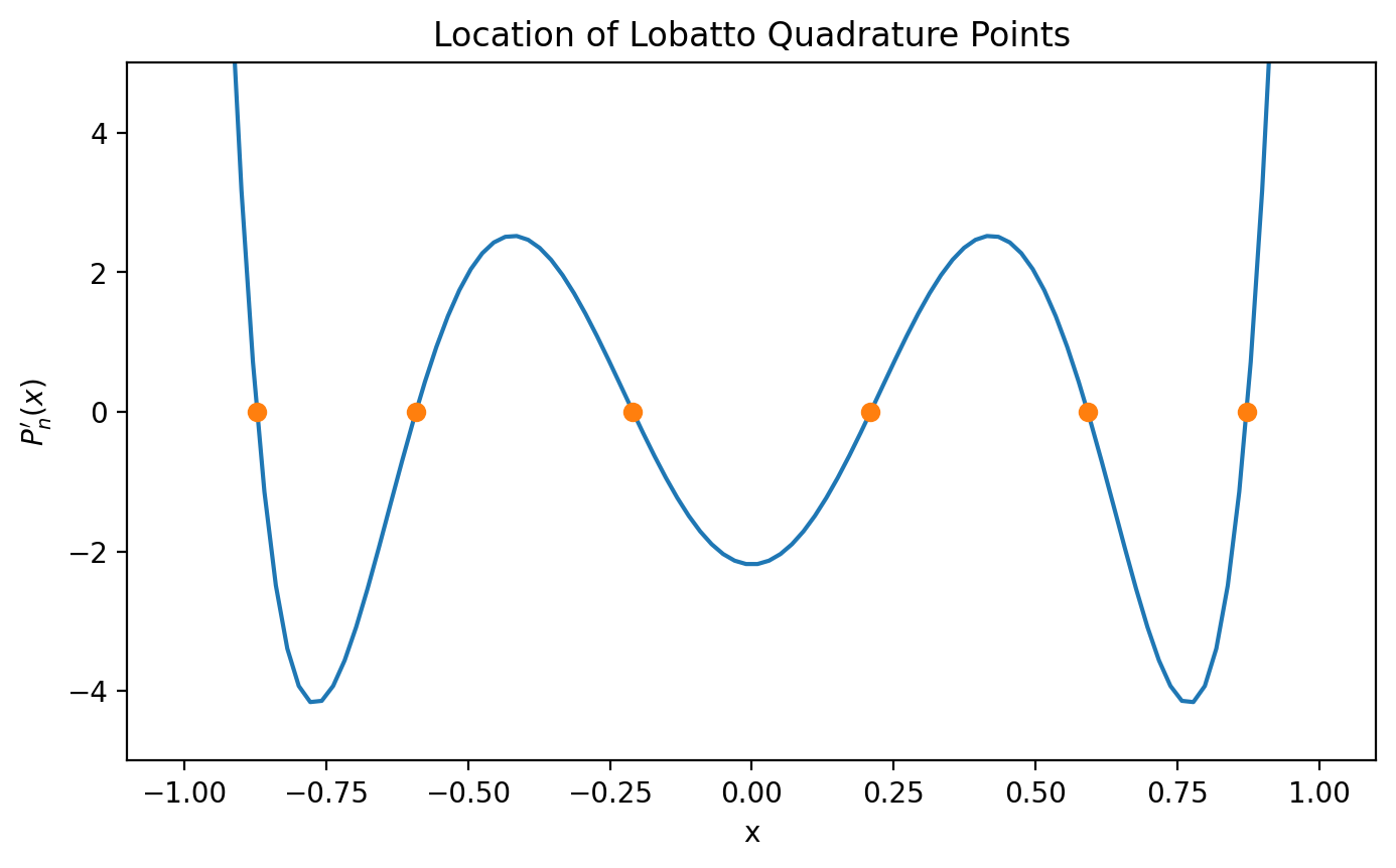
Gauss-Lobatto Quadrature
Gauss-Lobatto nodes are (except for the endpoints) the roots of \(P'_{n−1}(x)\).
[10]:
n=8
xi, wi = iadpython.quadrature.lobatto(n)
[11]:
xx=np.empty(8)
ww=np.empty(8)
xx[7]=-1
xx[6]=-0.8717401485096066153375
xx[5]=-0.5917001814331423021445
xx[4]=-0.2092992179024788687687
xx[3]=0.2092992179024788687687
xx[2]=0.5917001814331423021445
xx[1]=0.8717401485096066153375
xx[0]=1

ww[7]=0.03571428571428571428571
ww[6]=0.210704227143506039383
ww[5]=0.3411226924835043647642
ww[4]=0.4124587946587038815671
ww[3]=0.412458794658703881567
ww[2]=0.341122692483504364764
ww[1]=0.210704227143506039383
ww[0]=0.0357142857142857142857

xi = np.flip(xi)
print(" i        xi calc         xi ref            wi calc         wi ref")
print("----------------------------------------------------------------------")
for i,x in enumerate(xi):
    print("%2d   %+.12f %+.12f   %+.12f %+.12f" % (i, x, xx[i], wi[i], ww[i]))
 i        xi calc         xi ref            wi calc         wi ref
----------------------------------------------------------------------
 0   +1.000000000000 +1.000000000000   +0.035714285714 +0.035714285714
 1   +0.871740148510 +0.871740148510   +0.210704227144 +0.210704227144
 2   +0.591700181433 +0.591700181433   +0.341122692484 +0.341122692484
 3   +0.209299217902 +0.209299217902   +0.412458794659 +0.412458794659
 4   -0.209299217902 -0.209299217902   +0.412458794659 +0.412458794659
 5   -0.591700181433 -0.591700181433   +0.341122692484 +0.341122692484
 6   -0.871740148510 -0.871740148510   +0.210704227144 +0.210704227144
 7   -1.000000000000 -1.000000000000   +0.035714285714 +0.035714285714
[12]:
eps = 1e-8
x = np.linspace(-1+eps, 1-eps, 100)

plt.plot(x, iadpython.quadrature._lobatto_func(n,x))
plt.plot(xi[1:-1], iadpython.quadrature._lobatto_func(n,xi[1:-1]), "o")
plt.ylim(-5,5)
plt.xlabel("x")
plt.ylabel("$P_n'(x)$")
plt.title('Location of Lobatto Quadrature Points')
plt.show()
[13]:
n=10
xi, wi = iadpython.quadrature.lobatto(n,-7,2)

# integral of x^15 is (x**16)/16

quad_int = np.sum(xi**15* wi)
anal_int = (2)**16 / 16 - (-7)**16 / 16

print(quad_int)
print(anal_int)
-2077058156504.0247
-2077058156504.0625
[ ]: