Integrating Sphere Basics

Scott Prahl

Dec 2021

import numpy as np
import matplotlib.pyplot as plt

import iadpython.sphere
%config InlineBackend.figure_format='retina'

Integrating spheres are used to collect all light

The interior surfaces are a matte white paint (in the past this was something very white like MgSO₄ or BaSO₄). Any light entering the sphere will bounce around multiple times. Each bounce diffuses the incident light and it does this until the light fall on the inside walls of the sphere is uniform everywhere. A detector port can then be placed anywhere on the sphere to get a measure that scales with the total amount of light entering the sphere.

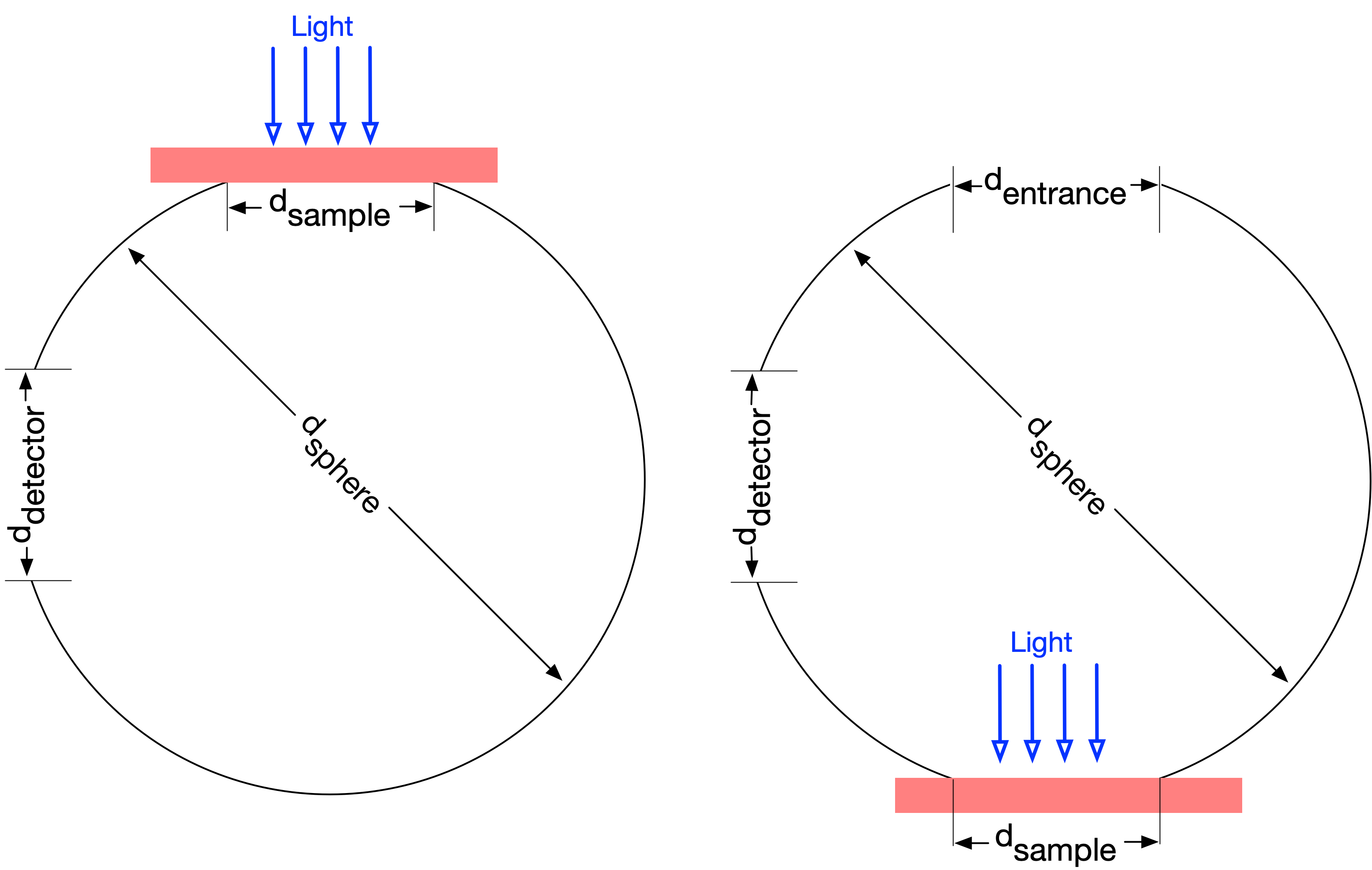
Port areas

If we look at a cross-section of an integrating sphere used in to measure transmission (left) and reflection (right) then we can see the diameters of the sphere and each of the ports.

The natural thing would be to use subscripts and define the relative area of the sample as \(a_\mathrm{sample}\). Relative area parameters are

\[a_\mathrm{sample} = \frac{\mbox{Area of sample port}}{\mbox{Surface area of integrating sphere}}\]

Other relative areas are the area of the detector \(a_\mathrm{detector}\), the area of the entrance port \(a_\mathrm{entrance}\), and the area of the sphere wall \(a_\mathrm{wall}\)

The total sphere surface includes the sphere has wall and ports (sample, detector, and entrance). Thus

\[A_\mathrm{total} = A_\mathrm{wall} + A_\mathrm{sample} + A_\mathrm{detector} + A_\mathrm{entrance}\]

or in terms of dimensionless relative areas

\[a_\mathrm{wall} = 1 - a_\mathrm{sample} - a_\mathrm{detector} - a_\mathrm{entrance}\]

One thing to note is that for the sphere on the left (the transmission experiment) the entrance port does not exist and therefore has zero area. The fraction of the sphere walls that is covered by ports is greater in the experiment on the left than the one on the right. Thus the relative wall area \(a_\mathrm{wall}\) for the two experiments will be different.

Spherical caps

The ports consist of holes in the sphere created by a plane passing through the edge of the sphere. This means that the area of the disk \(\pi a^2\) differs slightly from the area of the subtended surface area of sphere that was removed. This section is for those who worry about such things.

Note that a port with radius \(a\) has a cap area on a sphere with radius \(r\)

\[A_\mathrm{cap} = 2\pi r h\]

where \(h\) is the height of the cap

\[h = r - \sqrt{r^2-a^2}\]

The relative area is then

\[a_\mathrm{cap} = \frac{2\pi r h}{4\pi r^2} = \frac{r - \sqrt{r^2-a^2}}{2r} \approx \frac{a^2}{4r^2} - \frac{a^4}{16r^4} + \cdots\]

This can be compared directly with the normalized area of a disk divided by the surface area of the sphere:

\[a_\mathrm{cap}' = \frac{\pi a^2}{4\pi r^2} = \frac{a^2}{4r^2} = \frac{d_\mathrm{cap}^2}{4d_\mathrm{sphere}^2}\]

This is a tiny change from the naive approach; since \(a_\mathrm{cap}<0.01\) typically, the cap area error will be less than 1%.

Super simple sphere model: No reflection from ports

The simplest thing is to assume that the ports completely absorb any light that falls on them. Consider the case of a beam of light (P₀) that hits the wall and becomes perfectly diffuse,

\[\mbox{first bounce} = P_0 r_0\]

This light then falls on all the sphere walls. The total light reflected by the walls after this first bounce will be

\[\mbox{second bounce} = (P_0 r_0) \times (r_\mathrm{wall} a_\mathrm{wall})\]

this light will then be reflected again and the light hitting all walls for the second bounce will be

\[\mbox{third bounce} = (P_0 r_0) \times (r_\mathrm{wall} a_\mathrm{wall}) \times (r_\mathrm{wall} a_\mathrm{wall})\]

The total power on the walls will be

\[P_\mathrm{wall} = \mbox{(power from first bounce)} + \mbox{(power from second bounce)} + \cdots\]

or

\[P_\mathrm{wall} = P_0 r_0(1 + (r_\mathrm{wall}a_\mathrm{wall}) + (r_\mathrm{wall}a_\mathrm{wall})^2 + \cdots) = \frac{r_\mathrm{wall}}{1-r_\mathrm{wall}a_\mathrm{wall}} P_0\]

This suggests introducing a sphere multiplier \(M\) defined as

\[M = \frac{P_\mathrm{wall}}{P_0} = \frac{r_0}{1-r_\mathrm{wall}a_\mathrm{wall}}\]

and if the light hits the sphere wall first \(r_0=r_\mathrm{wall}\) so

\[M = \frac{r_\mathrm{wall}}{1-r_\mathrm{wall}a_\mathrm{wall}}\]

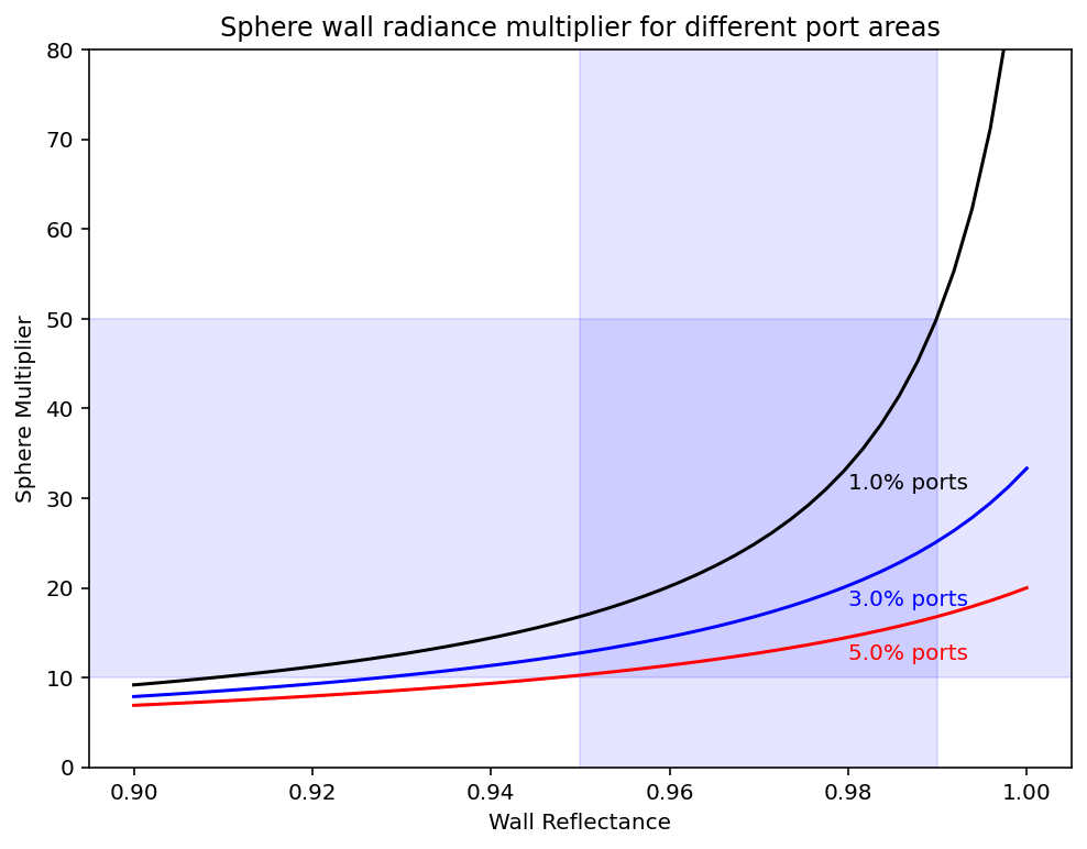
Sphere wall radiance multiplier for different port areas

There 10-50X more light on any part of the sphere wall than you would get if you just took the light entering the sphere and divided by the surface area of the walls. Here we see the how the two light loss mechanisms (port size and wall reflectance) affect this multipler.

sphere_diameter = 250
r_wall = np.linspace(0.9,1,50)
s = iadpython.sphere.Sphere(sphere_diameter, 1)

plt.figure(figsize=(8,6))

s.a_wall = 0.99
plt.plot(r_wall, s.multiplier(UR1=1, URU=0, r_wall=r_wall), color='black')
plt.text(0.98, 31, '%.1f%% ports'%(100-100*s.a_wall),color='black')

s.a_wall = 0.97
plt.plot(r_wall, s.multiplier(UR1=1, URU=0, r_wall=r_wall), color='blue')
plt.text(0.98, 18, '%.1f%% ports'%(100-100*s.a_wall),color='blue')

s.a_wall = 0.95
plt.plot(r_wall, s.multiplier(UR1=1, URU=0, r_wall=r_wall), color='red')
plt.text(0.98, 12, '%.1f%% ports'%(100-100*s.a_wall),color='red')

plt.xlabel('Wall Reflectance')
plt.ylabel('Sphere Multiplier')
plt.ylim(0,80)

plt.axvspan(0.95,0.99,color='blue',alpha=0.1)
plt.axhspan(10,50,color='blue',alpha=0.1)

plt.title("Sphere wall radiance multiplier for different port areas")

plt.show()

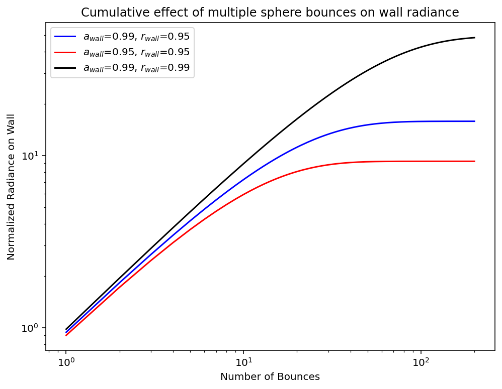
Cumulative effect of multiple sphere bounces on wall radiance

Each bounce contributes a little more. Highly reflective spheres with small port areas will bounce around hundreds of times before reaching a steady state radiance on the wall.

bounces = np.linspace(1,200,200)
plt.figure(figsize=(8,6))

a_wall = 0.99
r_wall = 0.95
r_cum = np.cumsum((r_wall*a_wall)**bounces)
label = '$a_{wall}$=%.2f, $r_{wall}$=%.2f'%(a_wall,r_wall)
plt.loglog(bounces, r_cum, 'b', label=label)

a_wall = 0.95
r_wall = 0.95
r_cum = np.cumsum((r_wall*a_wall)**bounces)
label = '$a_{wall}$=%.2f, $r_{wall}$=%.2f'%(a_wall,r_wall)
plt.loglog(bounces, r_cum, 'r', label=label)

a_wall = 0.99
r_wall = 0.99
r_cum = np.cumsum((r_wall*a_wall)**bounces)
label = '$a_{wall}$=%.2f, $r_{wall}$=%.2f'%(a_wall,r_wall)
plt.loglog(bounces, r_cum, 'k', label=label)

plt.legend()
plt.xlabel('Number of Bounces')
plt.ylabel('Normalized Radiance on Wall')
plt.title('Cumulative effect of multiple sphere bounces on wall radiance')
plt.show()

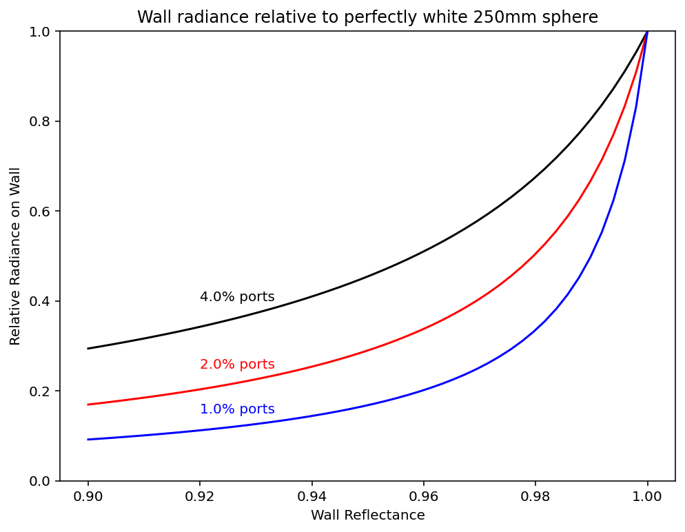
Wall radiance relative to perfectly white 250mm sphere

This is another graph showing the non-linear relationship between the wall radiance and the reflectivity of the sphere walls.

r_wall = np.linspace(0.9,1,50)
s = iadpython.sphere.Sphere(250, 1)
plt.figure(figsize=(8,6))

s.a_wall = 0.96
M = s.multiplier(UR1=1, URU=0, r_wall=r_wall)
plt.plot(r_wall, M/np.max(M),color='black')
plt.text(0.92, 0.4, '%.1f%% ports'%(100-100*s.a_wall),color='black')

s.a_wall = 0.98
M = s.multiplier(UR1=1, URU=0, r_wall=r_wall)
plt.plot(r_wall, M/np.max(M),color='red')
plt.text(0.92, 0.25, '%.1f%% ports'%(100-100*s.a_wall),color='red')

s.a_wall = 0.99
M = s.multiplier(UR1=1, URU=0, r_wall=r_wall)
plt.plot(r_wall, M/np.max(M),color='blue')
plt.text(0.92, 0.15, '%.1f%% ports'%(100-100*s.a_wall),color='blue')

plt.xlabel('Wall Reflectance')
plt.ylabel('Relative Radiance on Wall')
plt.ylim(0,1)
plt.title('Wall radiance relative to perfectly white 250mm sphere')

plt.show()