Single integrating sphere measurements

Scott Prahl

Dec 2021

import numpy as np
import matplotlib.pyplot as plt

import iadpython.sphere
%config InlineBackend.figure_format='retina'

Substitution vs Replacement Measurements

Integrating spheres are most easily used to make relative (rather than absolute) measurements. The total reflected light from a sample is compared to a standard or to the light hitting the sphere wall directly.

This section will calculate the measured relative value for a particular experiment.

Definitions

If we look at a cross-section of an integrating sphere used in to measure transmission (left) and reflection (right) then we can see the diameters of the sphere and each of the ports.

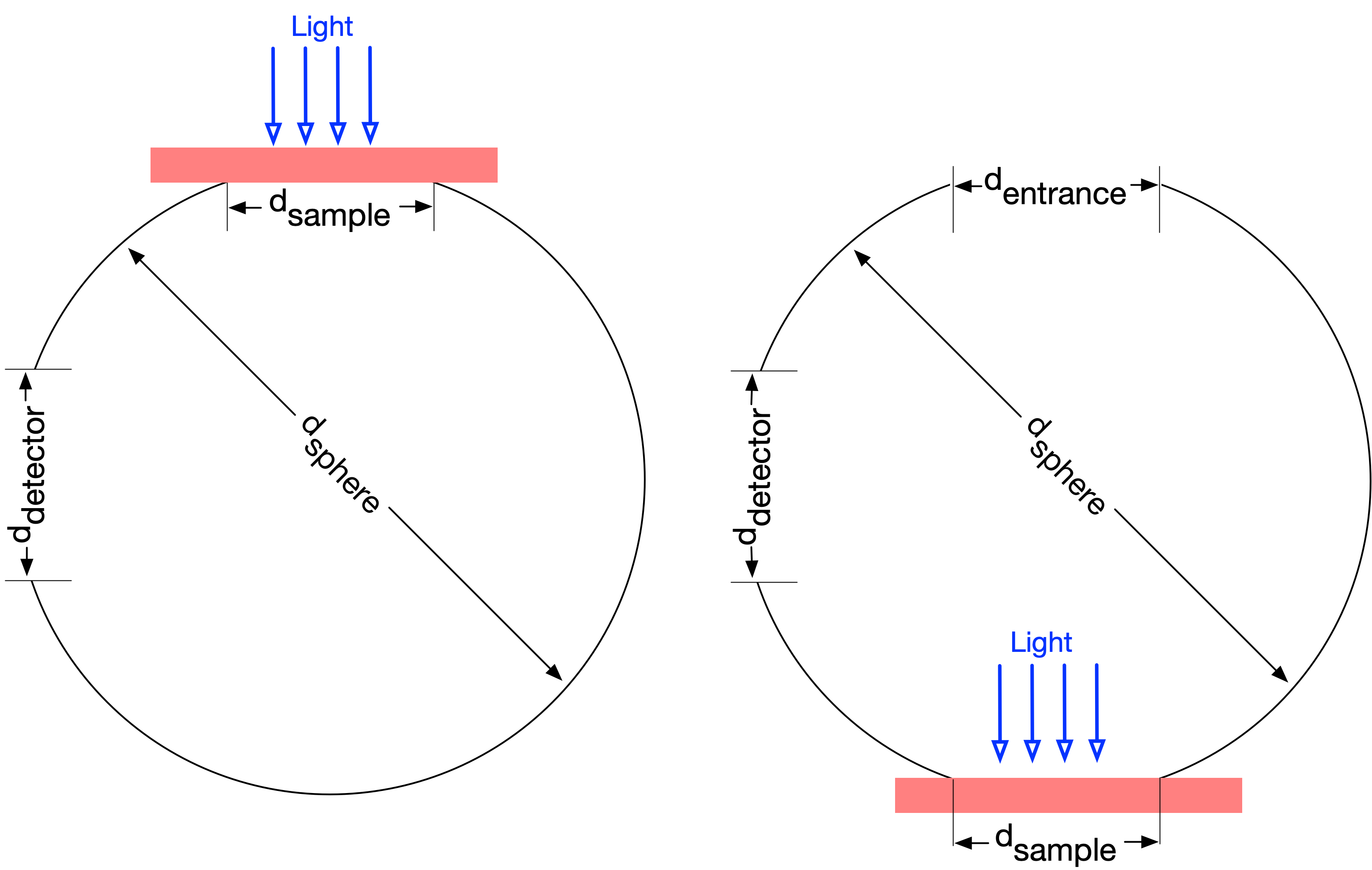
The natural thing would be to use subscripts and define the relative area of the sample as \(a_\mathrm{sample}\). Relative area parameters are

\[a_\mathrm{sample} = \frac{\mbox{Area of sample port}}{\mbox{Surface area of integrating sphere}}\]

Other relative areas are the area of the detector \(a_\mathrm{detector}\), the area of the entrance port \(a_\mathrm{entrance}\), and the area of the sphere wall \(a_\mathrm{wall}\)

The total sphere surface includes the sphere has wall and ports (sample, detector, and entrance). Thus

\[A_\mathrm{total} = A_\mathrm{wall} + A_\mathrm{sample} + A_\mathrm{detector} + A_\mathrm{entrance}\]

or in terms of dimensionless relative areas

\[a_\mathrm{wall} = 1 - a_\mathrm{sample} - a_\mathrm{detector} - a_\mathrm{entrance}\]

One thing to note is that for the sphere on the left (the transmission experiment) the entrance port does not exist and therefore has zero area. The fraction of the sphere walls that is covered by ports is greater in the experiment on the left than the one on the right. Thus the relative wall area \(a_\mathrm{wall}\) for the two experiments will be different.

Simple sphere model with sample and detector ports

The reflectance of each the ports is not usually 0%. Of course, the entrance port is remains empty and still has no reflectance. However, there is nearly always a sample and a detector. If we include these when calculating the total light then we get slightly different equations.

We start with a power \(P_0\) entering the sphere.

\[\mbox{first bounce} = r_0 P_0\]

The value of r₀ varies with the experiment. If the light is collimated, it might hit the sphere wall or a sample or it might pass through the a sample and emerge diffuse. It is also possible that the light enters the sphere fully diffuse. Some possible cases are

r₀	Description
1	fully diffuse light enters the sphere
r\(_w\)	light hits the walls of the sphere first
UR1	collimated light hits sample and is diffusely reflected into sphere
UT1	collimated light hits sample and is transmitted diffusely into sphere
URU	diffuse light hits sample and is diffusely reflected into sphere
UTU	diffuse light hits sample and is transmitted diffusely into sphere

This light \(r_0 P_0\) is assumed to be completely diffuse and reach all ports and walls in the sphere. The light reflected for the second bounce will be

\[\mbox{second bounce} = r_0 P_0 \cdot (r_\mathrm{wall} a_\mathrm{wall} + r_\mathrm{detector} a_\mathrm{detector} + r_\mathrm{sample} a_\mathrm{sample})\]

The second bounce is also totally diffuse and the third bounce will be

\[\mbox{third bounce} = r_0 P_0 \cdot (r_\mathrm{wall} a_\mathrm{wall} + r_\mathrm{detector} a_\mathrm{detector} + r_\mathrm{sample} a_\mathrm{sample})^2\]

Adding everything together, we get the total power on the walls

\[P_\mathrm{wall} = \frac{r_0 P_0}{1-(r_\mathrm{wall} a_\mathrm{wall} + r_\mathrm{detector} a_\mathrm{detector} + r_\mathrm{sample} a_\mathrm{sample})}\]

And so the sphere multiplier \(M\) above is modified to become

\[M = \frac{P_\mathrm{wall}}{P_0} = \frac{r_0}{1-(r_\mathrm{wall} a_\mathrm{wall} + r_\mathrm{detector} a_\mathrm{detector} + r_\mathrm{sample} a_\mathrm{sample})}\]

This means that the sample reflectance has a non-linear relationship to the reflectance. This gets worse when more internal bounces take place (i.e., as the port sizes get smaller for a constant wall reflectivity or as the reflectivity increases and the port sizes remain the same.) These effects are shown in the two graphs below.

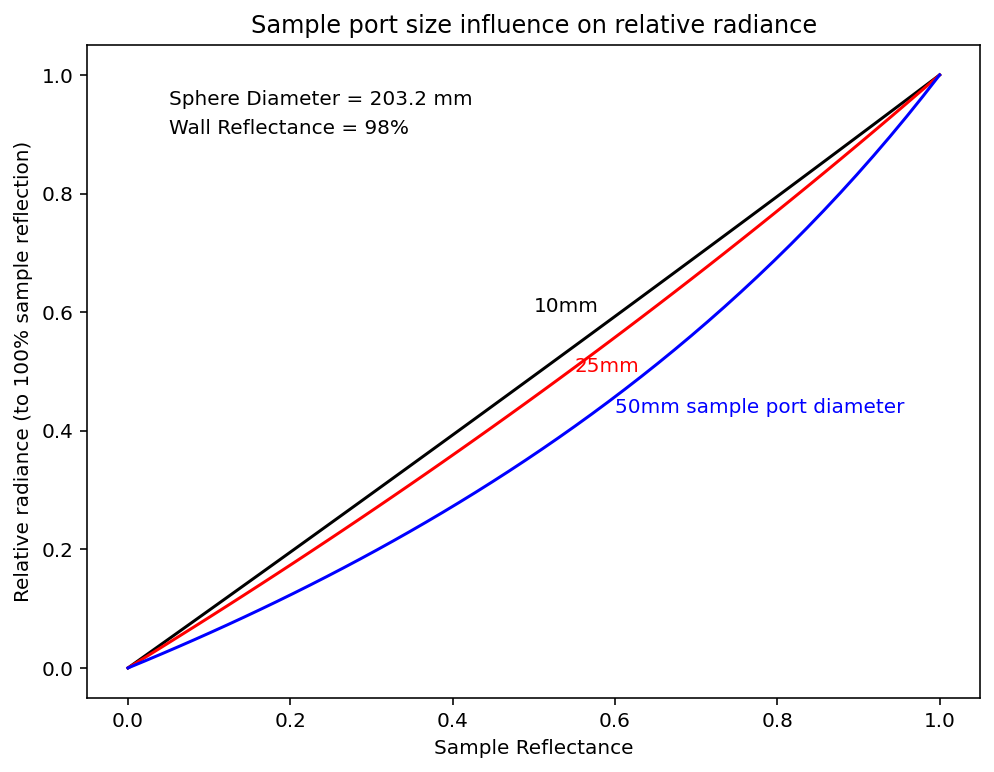
Effect of sample reflectance on relative radiance in sphere with 98% reflectivity

If the radiance on the walls of the sphere is linearly related to the reflectance (or transmittance) of a sample then we can just determine the sample reflectance with a few measurements \(M\)

\[R_\mathrm{sample} = \frac{M_s-M_0}{M_{100}-M_0}\]

However, as we can see below, as the sample size (i.e., port) gets larger and larger, this simple relationship breaks down.

r_sample = np.linspace(0.0,1,50)
s = iadpython.sphere.Sphere(25.4*8, 25.4, r_wall=0.98)

plt.figure(figsize=(8,6))

s.d_sample = 10
M = s.multiplier(UR1=r_sample, URU=r_sample)
plt.plot(r_sample, M/np.max(M), color='black')
plt.text(0.5,0.60,'%gmm'%(s.d_sample), color='black')

s.d_sample=25
M = s.multiplier(UR1=r_sample, URU=r_sample)
plt.plot(r_sample, M/np.max(M), color='red')
plt.text(0.55,0.5,'%gmm'%(s.d_sample), color='red')

s.d_sample=50
M = s.multiplier(UR1=r_sample, URU=r_sample)
label='$d_{sample}$=%.2f, %.0fmm sphere'%(s.a_wall,s.d_sphere)
plt.plot(r_sample, M/np.max(M), color='blue')
plt.text(0.6,0.43,'%gmm sample port diameter'%(s.d_sample), color='blue')

plt.xlabel('Sample Reflectance')
plt.ylabel('Relative radiance (to 100% sample reflection)')
plt.title('Sample port size influence on relative radiance')
plt.text(0.05,0.95,"Sphere Diameter = %g mm"%s.d_sphere)
plt.text(0.05,0.90,"Wall Reflectance = %g%%"%(100*s.r_wall))

plt.show()

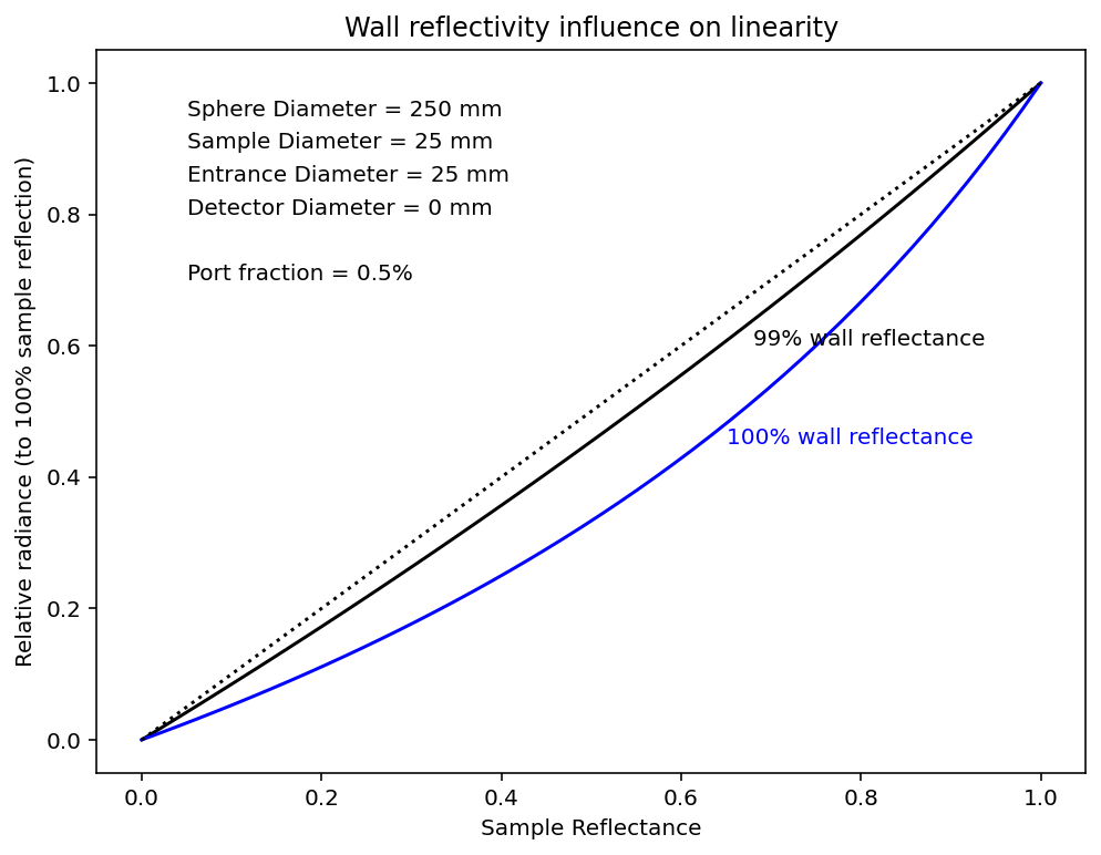
Effect of wall reflectivity on relative radiance with 25mm sample port

Here we see the slightly perplexing result that higher wall reflectivities increase non-linear response. This is follows from the fact that in whiter spheres, the light bounces around more times. The light has more chances to interact with the sample and therefore the sample ends up having a larger non-linear effect.

r_sample = np.linspace(0.0,1,50)
s = iadpython.sphere.Sphere(250, 25, d_entrance=25)

plt.figure(figsize=(8,6))

r_wall=0.99
M = s.multiplier(UR1=r_sample, URU=r_sample, r_wall=r_wall)

M100 = M[-1]
plt.plot(r_sample, M/M100, color='black')
plt.text(0.68,0.60,'%g%% wall reflectance'%(100*r_wall), color='black', ha='left')

r_wall=1.00
M = s.multiplier(UR1=r_sample, URU=r_sample, r_wall=r_wall)
plt.plot(r_sample, M/np.max(M), color='blue')
plt.text(0.65,0.45,'%g%% wall reflectance'%(100*r_wall), color='blue', ha='left')

plt.plot([0,1],[0,1],':k')
plt.xlabel('Sample Reflectance')
plt.ylabel('Relative radiance (to 100% sample reflection)')
plt.title('Wall reflectivity influence on linearity')
plt.text(0.05,0.95,"Sphere Diameter = %g mm"%s.d_sphere)
plt.text(0.05,0.90,"Sample Diameter = %g mm"%(s.d_sample))
plt.text(0.05,0.85,"Entrance Diameter = %g mm"%(s.d_entrance))
plt.text(0.05,0.80,"Detector Diameter = %g mm"%(s.d_detector))


plt.text(0.05,0.70,"Port fraction = %.2g%%"%(100-100*s.a_wall))

plt.show()

[ 0.          1.36863847  2.74669864  4.13427815  5.53147596  6.93839244
  8.35512934  9.78178985 11.21847858 12.66530166 14.12236669 15.58978281
 17.06766072 18.5561127  20.05525263 21.56519606 23.08606018 24.61796391
 26.16102787 27.71537449 29.28112794 30.85841427 32.44736137 34.04809902
 35.66075896 37.28547486 38.92238244 40.57161944 42.23332569 43.90764312
 45.59471587 47.29469024 49.00771479 50.73394038 52.47352019 54.2266098
 55.99336719 57.77395282 59.56852968 61.37726334 63.20032197 65.03787642
 66.89010028 68.75716992 70.63926454 72.53656623 74.44926005 76.37753408
 78.32157945 80.28159045]

1. what is gain

2. what is f

3. multiport analysis for UR1

4. multiport analysis for UT1

5. calculation of b1 and b2

6. calculation of sphere wall reflectivity

7. How much of an effect do these equations have??

Sphere model that tracks reflected sepa

Assume that a sphere is illuminated with diffuse light having a power P. Typically, the source of this diffuse light is light reflected by (or transmitted through) the sample.

We assume that this diffuse light can reach all parts of sphere — specifically, that light from this source is not blocked by a baffle. Multiple reflections within the sphere will increase the power falling on non-white areas in the sphere (e.g., the sample, detector, and entrance).

The total power entering the sphere is divided between the fractions hitting the wall, the sample port, the detector port, and the entrance port

\[P = P_\mathrm{wall} + P_\mathrm{sample} + P_\mathrm{detector} + P_\mathrm{entrance}\]

First incidence in reflection experiment

Consider a reflection experiment. In this case the light reflected by the sample P will only fall on the walls and the entrance port. It cannot hit the detector (because of a baffle) and it cannot hit the sample (because that is where it is leaving).

\[P_\mathrm{wall}^{(1)} = \frac{A_\mathrm{wall}}{A-A_\mathrm{detector}-A_\mathrm{sample}} P, \qquad P_\mathrm{sample}^{(1)} = 0, \qquad P_\mathrm{detector}^{(1)} = 0, \qquad P_\mathrm{entrance}^{(1)} = \frac{A_\mathrm{entrance}}{A-A_\mathrm{detector}-A_\mathrm{sample}} P\]

or (after dividing numerator and denominators in the fractions by \(A\)

\[P_\mathrm{wall}^{(1)} = \frac{a_\mathrm{wall}}{a_\mathrm{wall}+a_\mathrm{entrance}} P, \qquad P_\mathrm{sample}^{(1)} = 0, \qquad P_\mathrm{detector}^{(1)} = 0, \qquad P_\mathrm{entrance}^{(1)} = \frac{a_\mathrm{entrance}}{a_\mathrm{wall}+a_\mathrm{entrance}} P\]

We see that \(P=P_\mathrm{wall}^{(1)}+P_\mathrm{entrance}^{(1)}\). The light reflected

\[B_\mathrm{wall}^{(1)} = r_\mathrm{wall} P_\mathrm{wall}^{(1)}, \qquad B_\mathrm{sample}^{(1)} = 0, \qquad B_\mathrm{detector}^{(1)} = 0, \qquad B_\mathrm{entrance}^{(1)} = 0\]

First incidence in transmission experiment

Consider a transmission experiment. In this case the power transmitted by the sample P will only fall on the walls. It cannot hit the detector (because of a baffle), it cannot hit the entrance port (because there is none), and it cannot hit the sample (because that is where it is leaving). Thus all the light hits the walls

\[P_\mathrm{wall}^{(1)} = P, \qquad P_\mathrm{sample}^{(1)} = 0, \qquad P_\mathrm{detector}^{(1)} = 0, \qquad P_\mathrm{entrance}^{(1)} = 0\]

The light that bounces off the sphere parts is then

\[B_\mathrm{wall}^{(1)} = r_\mathrm{wall} P, \qquad B_\mathrm{sample}^{(1)} = 0, \qquad B_\mathrm{detector}^{(1)} = 0, \qquad B_\mathrm{entrance}^{(1)} = 0\]

Second incidence in reflection experiment

The distribution of power for the second incidence for each part can only arise from the first incidence on the walls

\[P_\mathrm{wall}^{(2)} = a_\mathrm{wall} B_\mathrm{wall}^{(1)}, \qquad P_\mathrm{sample}^{(2)} = a_\mathrm{sample} B_\mathrm{wall}^{(1)}, \qquad P_\mathrm{detector}^{(2)} = a_\mathrm{detector} B_\mathrm{wall}^{(1)}, \qquad P_\mathrm{entrance}^{(2)} = a_\mathrm{entrance} B_\mathrm{wall}^{(1)}\]

The second bounce from each part is then

\[B_\mathrm{wall}^{(2)} = r_\mathrm{wall}P_\mathrm{wall}^{(2)}, \qquad B_\mathrm{sample}^{(2)} = \mathrm{URU} \cdot P_\mathrm{sample}^{(2)}, \qquad B_\mathrm{detector}^{(2)} = r_\mathrm{detector} P_\mathrm{detector}^{(2)}, \qquad B_\mathrm{entrance}^{(2)} = 0\]

Third incidence in reflection experiment

The distribution of power for the third incidence for each part now arises from the first incidence on the walls

\[P_\mathrm{wall}^{(2)} = a_\mathrm{wall} (B_\mathrm{wall}^{(2)} + B_\mathrm{sample}^{(2)} + B_\mathrm{detector}^{(2)})\qquad P_\mathrm{sample}^{(2)} = a_\mathrm{sample} B_\mathrm{wall}^{(2)}\qquad P_\mathrm{detector}^{(2)} = a_\mathrm{detector} B_\mathrm{wall}^{(2)}, \qquad P_\mathrm{entrance}^{(2)} = a_\mathrm{entrance} (B_\mathrm{wall}^{(2)} + B_\mathrm{sample}^{(2)} + B_\mathrm{detector}^{(2)})\]

The second bounce from each part is then

\[B_\mathrm{wall}^{(2)} = r_\mathrm{wall}P_\mathrm{wall}^{(2)}, \qquad B_\mathrm{sample}^{(2)} = \mathrm{URU} \cdot P_\mathrm{sample}^{(2)}, \qquad B_\mathrm{detector}^{(2)} = r_\mathrm{detector} P_\mathrm{detector}^{(2)}, \qquad B_\mathrm{entrance}^{(2)} = 0\]

The light that hits the wall after \(k\) bounces has the same form as above

\[P_\mathrm{wall}^{(k)} = a_\mathrm{wall} r_\mathrm{wall} P_\mathrm{wall}^{(k-1)} + (1-a_\mathrm{entrance}) r_\mathrm{detector} P_\mathrm{detector}^{(k-1)} + (1-a_\mathrm{entrance}) r_\mathrm{sample} P_\mathrm{sample}^{(k-1)}\]

Since the light falling on the sample and detector must come from the wall

\[P_\mathrm{sample}^{(k)} = a_\mathrm{sample} r_\mathrm{wall} P_\mathrm{wall}^{(k-1)} \qquad\hbox{and}\qquad P_\mathrm{detector}^{(k)} = a_\mathrm{detector} r_\mathrm{wall} P_\mathrm{wall}^{(k-1)},\]

Therefore,

\[P_\mathrm{wall}^{(k)} = a_\mathrm{wall} r_\mathrm{wall} P_\mathrm{wall}^{(k-1)} + (1-a_\mathrm{entrance}) r_\mathrm{wall} (a_\mathrm{detector} r_\mathrm{detector} + a_\mathrm{sample} r_\mathrm{sample}) P_\mathrm{wall}^{(k-2)}\]

The total power falling on the wall is just

\[P_\mathrm{wall} = \sum_{k=1}^\infty P_\mathrm{wall}^{(k)} = \frac{a_\mathrm{wall} + (1-a_\mathrm{entrance}) ( a_\mathrm{detector} r_\mathrm{detector} +a_\mathrm{sample} r_\mathrm{sample})} {1- a_\mathrm{wall} r_\mathrm{wall} - (1-a_\mathrm{entrance})r_\mathrm{wall}(a_\mathrm{detector} r_\mathrm{detector} + a_\mathrm{sample} r_\mathrm{sample})} P\]

The total power falling the detector is

\[P_\mathrm{detector} = a_\mathrm{detector} P + \sum_{k=2}^\infty a_\mathrm{detector} r_\mathrm{wall} P_\mathrm{wall}^{(k-1)} = a_\mathrm{detector} P + a_\mathrm{detector} r_\mathrm{wall} P_\mathrm{wall}\]

The gain \(G(r_\mathrm{diffuse})\) on the irradiance on the detector (relative to a black sphere),

\[G(r_\mathrm{sample}) \equiv \frac{P_\mathrm{detector} /A_\mathrm{detector}}{P/A}\]

in terms of the sphere parameters

\[G(r_\mathrm{sample}) = 1+ {1\over a_\mathrm{wall}} \cdot {a_\mathrm{wall} r_\mathrm{wall} + (1-a_\mathrm{entrance}) r_\mathrm{wall} (a_\mathrm{detector} r_\mathrm{detector} +a_\mathrm{sample} r_\mathrm{sample}) \over 1- a_\mathrm{wall} r_\mathrm{wall} - (1-a_\mathrm{entrance})r_\mathrm{wall}(a_\mathrm{detector} r_\mathrm{detector} + a_\mathrm{sample} r_\mathrm{sample})}\]

The gain for a detector in a transmission sphere is similar, but with primed parameters to designate a second potential sphere that is used. For a black sphere the gain \(G(0) = 1\), which is easily verified by setting \(r_\mathrm{wall}=0\), \(r_\mathrm{diffuse}=0\), and \(r_\mathrm{detector}=0\). Conversely, when the sphere wall and sample are perfectly white, the irradiance at the entrance port, the sample port, and the detector port must increase so that the total power leaving via these ports is equal to the incident diffuse power \(P\).

Thus the gain should be the ratio of the sphere wall area over the area of the ports through which light leaves or \(G(1)=A/(A_\mathrm{entrance}+A_\mathrm{detector})\) which follows immediately from the gain formula with \(r_\mathrm{wall}=1\), \(r_\mathrm{diffuse}=1\), and \(r_\mathrm{detector}=0\).

The gain \(G(r_\mathrm{sample})\) on the irradiance on the detector (relative to a black sphere),

\[G(r_\mathrm{sample}) \equiv {P_\mathrm{detector} /A_\mathrm{detector}\over P/A}\]

in terms of the sphere parameters

\[G(r_\mathrm{sample}) = 1+ {a_\mathrm{wall} r_\mathrm{wall} + (1-a_\mathrm{entrance}) r_\mathrm{wall} (a_\mathrm{detector} r_\mathrm{detector} +a_\mathrm{sample} r_\mathrm{sample}) \over 1- a_\mathrm{wall} r_\mathrm{wall} - (1-a_\mathrm{entrance})r_\mathrm{wall}(a_\mathrm{detector} r_\mathrm{detector} + a_\mathrm{sample} r_\mathrm{sample})}\]